Table of Contents

Open Table of Contents

• Policy as NN
• Policy Gradient Theorem & REINFORCE
• Baselines and Advantages
• Actor Critic and GAE
• Natural Policy Gradient
• TRPO
• PPO
• PPO in Practice: A Minimal Continuous-Control Update
  • 1. Define ActorCritic
  • 2. Sample an Action with the Old Policy
  • 3. Compute GAE and Critic Targets
  • 4. Re-evaluate Stored Actions and Update the Networks
  • 5. Read the Update Line by Line
  • 6. Bounded Actions: One Important Omission

Policy as NN

Policy based reinforcement learning aims to learn the “policy” itself. It parameterizes policy as a neural network $\theta$ and directly optimizes it unlike value-based reinforcement learning that usually learn a Q-value function and extract a deterministic policy afterwards (Q-learning, SARSA, DQN).

Some notations :

Meaning	Notation	Explanation
policy	$\pi_{\theta} (a_t \mid s_t)$	the action distribution under a certain state
reward	$r(s_t, a_t)$	the reward of taking an action at a state
trajectory	$\tau$	also known as an episode, $\tau = (s_1, a_1, \dots, s_t, a_t)$
value	$V^\pi(s)$	$V^\pi(s) = E_\pi \left[ \sum_{k=t}^{T} \gamma^{k-t}r_k \mid s_t=s \right]$
Q-value	$Q^\pi(s,a)$	$Q^\pi(s,a) = E_\pi \left[ \sum_{k=t}^{T} \gamma^{k-t}r_k \mid s_t=s , a_t=a\right]$

Policy Gradient Theorem & REINFORCE

A policy is optimal when the mean total reward of all trajectories sampled from the policy is the largest, so we define our target function as follows:

$$J(\theta) = \mathbb{E}_{\tau \sim p_{\theta(\tau)}}R(\tau) = \mathbb{E}_{\tau \sim p_{\theta(\tau)}} \left[ \sum_t r(s_t, a_t) \right]$$

here the likelihood of trajectory $\tau$ under policy $\pi_\theta$ is:

$$p_\theta(\tau) = p_\theta(s_0,a_1,\dots,s_t,a_t) = p(s_0)\prod_t \pi_\theta(a_t| s_t) p(s_{t+1} | s_t,a_t)$$

Now we want to find the $\theta^{\star}$ that maximize $J(\theta)$, we can calculate $\nabla_\theta J(\theta)$ and do gradient ascent to find the argmax. Policy Gradient Theorem has that:

$$\nabla_\theta J(\theta) = \mathbb{E}_{\tau \sim p_\theta{(\tau)}} \left[ R(\tau) \sum_t \nabla_\theta \log{\pi_\theta(a_t| s_t)} \right]$$

Intuitively, this means that for a high-reward trajectory, we want the action in this trajectory to appear more frequently.

Expand to see the proof

$$\begin{aligned} \nabla_\theta J(\theta) &= \nabla_\theta\sum_{\tau}R(\tau)p_\theta(\tau) \\ &= \sum_{\tau} R(\tau)\nabla_\theta p_\theta(\tau) \\ &= \sum_{\tau}R(\tau)p_\theta(\tau) \nabla_\theta \log p_\theta(\tau) \quad \quad \color{red}\nabla f(x) = f(x)\nabla\log f(x)\\ &= \mathbb{E}_{p_\theta(\tau)}\left[ R(\tau) \nabla_\theta \log p_\theta(\tau)\right] \\ &= \mathbb{E}_{p_\theta(\tau)}\left[ R(\tau) \nabla_\theta \log \prod_t \pi_\theta(a_t| s_t) p(s_{t+1} | s_t,a_t)\right] \\ &= \mathbb{E}_{p_\theta(\tau)}\left[ \sum_t R(\tau) \nabla_\theta \left( \log \pi_\theta(a_t| s_t)+\log p(s_{t+1} | s_t,a_t)\right)\right] \\ &= \mathbb{E}_{p_\theta(\tau)}\left[ \sum_t R(\tau) \nabla_\theta \log \pi_\theta(a_t| s_t) \right] + \mathbb{E}_{p_\theta(\tau)}\left[\nabla_\theta \underbrace{\log p(s_{t+1} | s_t,a_t)}_{\text{independent of } \theta}\right] \\ &= \mathbb{E}_{p_\theta(\tau)}\left[ \sum_t R(\tau) \nabla_\theta \log \pi_\theta(a_t| s_t) \right] \end{aligned}$$

And this leads to REINFORCE, the simplest policy gradient algorithm — use Monte Carlo to estimate $\nabla_\theta J(\theta)$ and use gradient ascent on it：

1. Sample $\{ \tau^i \}$ from policy $\pi_\theta$
2. $\nabla_\theta J(\theta) = \frac{1}{N} \sum_i \left[ (\sum_t r(a_t^i, s_t^i)) (\sum_t \nabla_\theta \log{\pi_\theta(a_t^i| s_t^i)}) \right]$
3. $\theta \leftarrow \theta + \alpha \nabla_\theta J(\theta)$

Baselines and Advantages

Standard PG usually has very large variance. This is because we update action over the overall reward of the whole sampled trajectory, the super-long rollout adds to stochasticity and variance. One way to reduce the variance is to shorten the reward horizon. Notice that there is causality within the PG theorem that action at time $t^{\prime}$ cannot affect reward at $t < t^\prime$, so reward in the part won’t affect current policy.

$$\begin{aligned} \nabla_\theta J(\theta) &= \mathbb{E}_{\tau \sim p_\theta{(\tau)}} \left[ (\sum_t \nabla_\theta \log{\pi_\theta(a_t^i| s_t^i)}) (\sum_t r(a_t^i, s_t^i)) \right] \\ &= \mathbb{E}_{\tau \sim p_\theta{(\tau)}} \left[ \sum_t (\nabla_\theta \log{\pi_\theta(a_t^i| s_t^i)} \underbrace{(\sum_{t^\prime = t} r(a_{t^\prime}^i, s_{t^\prime}^i)))}_{ \text{Reward to go}} \right] \quad\quad \quad \end{aligned}$$

Notice that $Q^{\pi}(s, a) = \mathbb{E}_{\pi}\left[ \sum_{t'=t} \gamma^{t'-t} r_{t'} \mid s_t = s, a_t = a\right]$, which is expected discounted reward-to-go. So we have:

$$\nabla_\theta J(\theta) \propto \mathbb{E}_{\tau \sim p_\theta{(\tau)}} \left[\sum_t Q^\pi(s_t^i, a_t^i)\nabla_\theta \log \pi_\theta (a_t^i | s_t^i) \right]$$

We can do a little reformulation for this equation. Averaging over trajectory samples and timestep is equal to taking expectation over the state-action visitation distribution, where we can introduce a state visitation distribution $d^\pi(s) = \sum_t P(s_t=s|\pi)$. So that we can have a neater expression for PG theorem:

$$\nabla_\theta J(\theta) = \mathbb{E}_{s \sim d^\pi(s), a\sim \pi} \left[ Q^\pi(s,a) \nabla_\theta \log{\pi_\theta(a| s)} \right]$$

Expand to see the proof

$$\begin{aligned} \nabla_\theta J(\theta) &= \mathbb{E}_{\tau\sim p_\theta(\tau)} \left[ \sum_{t=0}^{T} Q^\pi(s_t,a_t) \nabla_\theta\log\pi_\theta(a_t|s_t) \right] \\ &= \sum_{t=0}^{T} \mathbb{E}_{\tau\sim p_\theta(\tau)} \left[ Q^\pi(s_t,a_t) \nabla_\theta\log\pi_\theta(a_t|s_t) \right] \\ &= \sum_{t=0}^{T} \int_s\int_a p(s_t=s,a_t=a|\pi) Q^\pi(s,a) \nabla_\theta\log\pi_\theta(a|s) \,da\,ds \\ &= \sum_{t=0}^{T} \int_s\int_a p(s_t=s|\pi) \pi_\theta(a|s) Q^\pi(s,a) \nabla_\theta\log\pi_\theta(a|s) \,da\,ds \\ &\propto \int_s\int_a d^\pi(s) \pi_\theta(a|s) Q^\pi(s,a) \nabla_\theta\log\pi_\theta(a|s) \,da\,ds \\ &= \mathbb{E}_{s\sim d^\pi(s),\,a\sim\pi_\theta(a|s)} \left[ Q^\pi(s,a) \nabla_\theta\log\pi_\theta(a|s) \right]. \end{aligned}$$

Now we introduce the baseline method, subtracting an action-independent baseline does not affect the policy gradient as long as this bias term is not a function of $a$ :

$$\nabla_\theta J(\theta) \propto \mathbb{E}_{s\sim p_\theta{(s)}, a\sim \pi} \left[ (Q^\pi(s,a)-b(s)) \nabla_\theta \log{\pi_\theta(a| s)} \right]$$

Expand to see the proof

$$\begin{aligned} &\quad\mathbb{E}_{s\sim p_\theta{(s)}, a\sim \pi} \left[ b(s)\nabla_\theta \log{\pi_\theta(a| s)} \right] \\ &= \int_{s}\int_a d^\pi(s)\pi_\theta(a|s)b(s)\nabla_\theta \log{\pi_\theta(a| s)}dads\\ &= \int_{s}d^\pi(s)b(s)\int_a\pi_\theta(a|s)\nabla_\theta \log{\pi_\theta(a| s)}dads \\ &= \int_{s}d^\pi(s)b(s)\int_a\pi_\theta(a|s) \frac{\nabla_\theta\pi_\theta(a|s)}{\pi_\theta(a|s)}dads \\ &= \int_{s}d^\pi(s)b(s)\nabla_\theta \int_a \pi_\theta(a|s)dads \\ &= \int_{s}d^\pi(s)b(s)\nabla_\theta1dads = 0 \end{aligned}$$

Actor Critic and GAE

Now that we have the baseline theorem, we can move on to the actor-critic algorithm. $b(s)$ in the baseline theorem can be any function of state. The most common function of state in RL theory is the value function $V^\pi(s)$.

$$\nabla_\theta J(\theta) = \mathbb{E}_{s\sim p_\theta{(s)}, a\sim \pi} \left[ (Q^\pi(s,a)-V^\pi(s)) \nabla_\theta \log{\pi_\theta(a| s)} \right]$$

The intuition of the equation is also clear. The vanilla PG theorem uses the reward of entire trajectory to weigh every action. Actor-critic does this in a more fine-grained way. It weighs each action by how much more reward it can get than the average of all actions. This can be seen as an advantage of this action over the mean, so this term is also known as an advantage term.

$$A^\pi(s,a) = Q^\pi(s,a)-V^\pi(s)$$

Typically this $V^\pi(s)$ is another network (the critic in Actor-Critic), so we use $V^\pi_\phi(s)$ as its notation. We now need to know $Q$ to calculate the advantage. There are two simple ways.

The first is to use Monte Carlo method. Since $Q^\pi(s,a)$ is the expectation of Reward-to-Go, we then simply let $Q^\pi(s,a) \approx \sum_{k=t}^T\gamma^{k-t}r_{k}$. This method has low bias but huge variance since we introduce the entire trajectory. The second way is temporal difference. Instead of writing out the entire future trajectory, TD methods bootstrap from the critic: $Q^\pi(s,a) \approx r_t + \gamma V^\pi_\phi(s_{t+1})$. So the advantage can be written as $A^\pi(s,a) = r_t + \gamma V^\pi_\phi(s_{t+1}) -V^\pi_\phi(s_t)$. It has lower variance because it replaces most future rewards with a bootstrapped value estimate. Its error or bias comes from inaccuracies in the learned critic and, more generally, from function approximation and bootstrapping. The TD-error measures the gap between the critic’s current prediction and a one-step improved estimate.

GAE (Generalized Advantage Estimation) aims to strike a balance between the two methods. The core concept of GAE is to use a weighted sum of TD-errors to construct a low variance estimation for the advantage. The final expression is:

$$\hat A_t^{GAE(\gamma,\lambda)} = \sum_{l=0}^{\infty} (\gamma\lambda)^l \delta_{t+l}$$

where $\delta_t = r_t+\gamma V_\phi(s_{t+1})-V_\phi(s_t)$ is the TD-error, $T$ is the trajectory length and $\lambda$ controls between Monte Carlo estimation (low bias, high variance) and one-step TD (high bias, low variance). If $\lambda = 0$, $A_t = \delta_{t}$ becomes one-step TD. If $\lambda = 1$, it reduces to the Monte Carlo advantage estimate $R_t-V_\phi(s_t)$.

Expand to see the proof

Define n-step bootstrapped Q-value as.

$$\hat Q_t^{(n)} = \sum_{l=0}^{n-1}\gamma^l r_{t+l} + \gamma^{n}V^{\pi}_{\phi}(s_{t+n})$$

The corresponding $n$-step advantage estimate is

$$\hat A_t^{(n)} = \hat Q_t^{(n)}-V_\phi(s_t)$$

For $n=1$,

$$\begin{aligned} \hat A_t^{(1)} &= r_t+\gamma V_\phi(s_{t+1})-V_\phi(s_t) = \delta_t \end{aligned}$$

For $n=2$,

$$\begin{aligned} \hat A_t^{(2)} &= r_t + \gamma r_{t+1} + \gamma^2 V_\phi(s_{t+2}) -V_\phi(s_t) \\ &= (r_t + \gamma V_\phi(s_{t+1})-V_\phi(s_t)) + (\gamma r_{t+1} + \gamma^2 V_\phi(s_{t+2}) - \gamma V_\phi(s_{t+1})) \\ &= \delta_t + \gamma \delta_{t+1}\end{aligned}$$

Similarly, in general, $\hat A_t^{(n)} = \sum_{l=0}^{n-1} \gamma^{l}\delta_{t+l}$ Now we want to weighted sum all n-step advantages

$$\begin{aligned} \hat A^{GAE}_t &= (1-\lambda)\sum_{n=1}^{\infty}\lambda^{(n-1)} \hat A_t^{(n)} \\ &= (1-\lambda)\sum_{n=1}^{\infty}\lambda^{(n-1)} \sum_{l=0}^{n-1} \gamma^{l}\delta_{t+l} \end{aligned}$$

Interchange the order of summation, we have

$$\begin{aligned} \hat A^{GAE}_t &= (1-\lambda) \sum_{l=0}^{\infty} \gamma^{l} \left(\sum_{n=l}^{\infty}\lambda^n\right) \delta_{t+l} \\ &= \sum_{l=0}^{\infty}(\gamma \lambda)^l \delta_{t+l} \end{aligned}$$

For finite trajectory, we have:

$$\begin{aligned} \hat A^{GAE}_t &= (1-\lambda)\sum_{n=1}^{T-t+1}\lambda^{(n-1)} \sum_{l=0}^{n-1} \gamma^{l}\delta_{t+l} \\ &= (1-\lambda) \sum_{l=0}^{T-t}\gamma^{l}\left(\sum_{n=l}^{T-t}\lambda^{n}\right)\delta_{t+l} \\ &= \sum_{l=0}^{T-t}\gamma^{l} \lambda^{l}(1-\lambda^{T-t-l+1})\delta_{t+l} \\ &= \sum_{l=0}^{T-t}(\gamma\lambda)^{l}\delta_{t+l} - \underbrace{\lambda^{T-t+1}\sum_{l=0}^{T-t}\gamma^l \delta_{t+l}}_{\text{finite-horizon correction term}} \end{aligned}$$

The above derivation proves the equivalence between GAE and the exponentially weighted average of n-step advantages under an infinite horizon. In practice, GAE is usually implemented recursively:

$$\hat A_t=\delta_t+\gamma\lambda\hat A_{t+1}$$

Expanding the recursion gives:

$$\hat A_t = \sum_{l=0}^{\infty} (\gamma\lambda)^l\delta_{t+l}$$

For infinite trajectories, this formulation is equivalent to the weighted n-step formulation. For finite trajectories, however, truncating the trajectory introduces different boundary effects depending on the formulation.

In the recursive implementation, the boundary effect appears through the last TD error:

$$\delta_T=r_T+\gamma V_\phi(s_{T+1})-V_\phi(s_T)$$

If the trajectory terminates naturally, $V_\phi(s_{T+1})=0$. If the trajectory is truncated due to a time limit, $V_\phi(s_{T+1})$ is retained for bootstrapping.

Natural Policy Gradient

Now let’s move on to the next stage. Both PG and Actor-Critic update parameter with gradient ascend $\theta \leftarrow \theta + \alpha\nabla_\theta J(\theta)$, where $\alpha$ is the learning rate. This update rule works well in supervised learning because the training labels are fixed, independent of the model being optimized. However, reinforcement learning is different: the learning signal itself depends on the current policy, since the collected trajectories and future rewards are generated by the policy being optimized. If learning rate is too big, the policy may “overshoot” to a region with worse performance. Since future training data are collected by this degraded policy, the learning signal can become less informative or even misleading, making recovery difficult. Using a very small learning rate makes training stable but inefficient. This can be more easily understood by formulating the gradient ascent as a optimization problem.

$$\begin{aligned} \max_{\theta'}\quad & (\theta'-\theta)^T\nabla_\theta J(\theta) \\ \text{s.t.}\quad & \|\theta-\theta'\|^2\leq\epsilon \end{aligned}$$

This means “Among all possible new parameters within a small neighborhood of the current policy, which direction gives the largest improvement in the objective?” This formulation is equivalent to the gradient ascending expression and the $\epsilon$ here is proportional to learning rate $\alpha$.

The problem arises in the 2-norm constraint. Proximity in parameter space does not necessarily mean proximity in policy space. Also, different directions in parameter space can have different effects on the resulting policy distribution. For the same numerical change, some dimension introduces greater changes than others. The $L_2$ norm only measures the magnitude of parameter changes and assumes that changes in all directions have the same importance. Therefore, we need a metric that measures the distance between policies rather than parameters. We can use the KL-divergence between old and new policy as the constraint.

$$\begin{aligned} \max_{\theta'}\quad & (\theta'-\theta)^T\nabla_\theta J(\theta) \\ \text{s.t.}\quad & D_{KL}(\pi_\theta||\pi_{\theta'})\leq\epsilon \end{aligned}$$

KL distance can be expressed in Fisher information matrix when $\Delta\theta$ is around zero. $D_{KL} \approx \frac12 \Delta\theta^T F \Delta\theta$, where $F = E [ \nabla_\theta\log\pi \nabla_\theta\log\pi^T ]$, so the optimization problem becomes,

$$\begin{aligned} \max_{\theta'}\quad & (\theta'-\theta)^T\nabla_\theta J(\theta) \\ \text{s.t.}\quad & \frac12 \Delta\theta^TF\Delta\theta \leq\epsilon \end{aligned}$$

Solve this constrain problem and we can have the gradient update formula: $\theta^\prime \leftarrow \theta + \alpha F^{-1}\nabla J$. This method is called Natural Gradient.

Although natural gradient provides a more principled update direction, it still has several limitations. First, the derivation relies on a local quadratic approximation of the KL divergence. For large updates, this approximation can become inaccurate, causing the actual policy change to exceed the desired trust region. Second, the Fisher information matrix is expensive to compute and store for large neural networks, making direct matrix inversion impractical. Finally, natural gradient does not explicitly verify whether the update improves the policy, since the theoretical guarantee only holds under local assumptions, namely $J(\theta+\Delta\theta)$ is not necessarily greater than $J(\theta)$.

TRPO

This is where TRPO comes into play. We first need a view shift. Let’s first review the basics. Both vanilla PG and natural gradient tries to solve the following optimization problem.

$$\max_\theta \space J(\theta)$$

There are two different perspectives to understand this optimization problem.

The first perspective is the gradient optimization view: starting from the current policy $\pi_\theta$, we iteratively update its parameters according to the estimated gradient:

$$\theta\leftarrow\theta+\alpha\nabla_\theta J(\theta)$$

This is the perspective vanilla policy gradient and natural gradient takes.

TRPO and PPO take the policy improvement perspective: given a current policy $\pi_\theta$, we search for a new policy $\pi_{\theta'}$ that improves upon it:

$$J(\theta')-J(\theta)>0$$

In this new perspective, we can directly perform $\max_{\theta'} \space J(\theta')-J(\theta)$ to improve the policy. We first write out the detailed formulation of this target term

$$J(\theta') - J(\theta) = \mathbb{E}_{\tau\sim p_{\theta'}(\tau)} \left[ \sum_t \gamma^t A^{\pi_\theta}(s_t, a_t)\right]$$

Expand to see full derivation

First, we expand $J(\theta)$

$$J(\theta) = \mathbb{E}_{s_0 \sim p(s_0)}\left[ V^{\pi_\theta}(s_0) \right] = \mathbb{E}_{\tau \sim p_{\theta'}(\tau)}\left[V^{\pi_\theta}(s_0)\right]$$

The first equation is because $V^{\pi_\theta}(s_0) = E_\pi \left[ \sum_{k=t}^{T} \gamma^{k-t}r_k \mid s_t=s \right]$ and the expectation averages over all initial states; the second equation is because $V^{\pi_\theta}(s_0)$ is only dependent on $s_0$ instead of the whole trajectory, and the marginal distribution of $s_0$ from $p_{\theta'}(\tau)$ is still from $p(s_0)$.

Then we use a trick called telescoping sum,

$$J(\theta) = \mathbb{E}_{\tau \sim p_{\theta'}(\tau)}\left[\sum_{t=0}\gamma^{t}V^{\pi_\theta}(s_t) - \sum_{t=1}\gamma^{t}V^{\pi_\theta}(s_t)\right]$$

Now get in the original target and rearrange the terms,

$$\begin{aligned} J(\theta') - J(\theta) &= J(\theta') - \mathbb{E}_{\tau \sim p_{\theta'}(\tau)}\left[\sum_{t=0}\gamma^{t}V^{\pi_\theta}(s_t) - \sum_{t=1}\gamma^{t}V^{\pi_\theta}(s_t)\right] \\ &= J(\theta') + \mathbb{E}_{\tau \sim p_{\theta'}(\tau)}\left[\sum_{t=0}\gamma^{t}(\gamma V^{\pi_\theta}(s_{t+1}) - V^{\pi_\theta}(s_{t}))\right] \\ &= \mathbb{E}_{\tau \sim p_{\theta'}(\tau)}\left[\sum_{t=0}\gamma^t r(s_t,a_t)\right] + \mathbb{E}_{\tau \sim p_{\theta'}(\tau)}\left[\sum_{t=0}\gamma^{t}(\gamma V^{\pi_\theta}(s_{t+1}) - V^{\pi_\theta}(s_{t}))\right] \\ &= \mathbb{E}_{\tau \sim p_{\theta'}(\tau)}\left[\sum_{t=0}\gamma^{t}(r(s_t,a_t) + \gamma V^{\pi_\theta}(s_{t+1}) - V^{\pi_\theta}(s_{t}))\right] \\ &= \mathbb{E}_{\tau \sim p_{\theta'}(\tau)}\left[\sum_{t=0}\gamma^{t}(Q^{\pi_\theta}(s_t,a_t) - V^{\pi_\theta})(s_t)\right] \\ &= \mathbb{E}_{\tau \sim p_{\theta'}(\tau)}[\sum_{t=0}\gamma^{t} A^{\pi_\theta}(s_t,a_t)] \end{aligned}$$

Although the derivation is somewhat involved, the resulting identity has a simple interpretation. It means that “the new policy is better than the old policy if it increases the probability of actions that are better than what the old policy expected.” The RHS can be viewed as how much the new policy improves over the old policy by accumulating the advantages of the actions taken by the new policy.

But we can’t directly optimize this target since the expectation is taken over the new policy distribution. We can’t sample from a policy if we haven’t known the policy. So the core idea of TRPO (and also PPO) is that can we use $\mathbb{E}_{\tau\sim p_{\theta}(\tau)}$ to optimize $J(\theta') - J(\theta)$ by controlling the distance between $\theta$ and $\theta'$. (i.e. can we collect data from old policy to get a new policy).

We first use importance sampling to reformulate the term

$$\begin{aligned} J(\theta') - J(\theta) &= \mathbb{E}_{\tau\sim p_{\theta'}(\tau)} \left[ \sum_t \gamma^t A^{\pi_\theta}(s_t, a_t)\right] \\ &= \sum_t \mathbb{E}_{\tau\sim p_\theta'(\tau)} \left[ \gamma^t A^{\pi_\theta}(s_t, a_t)\right] \\ &= \sum_t \mathbb{E}_{(s_t,a_t)\sim p_\theta'(s_t,a_t)} \left[ \gamma^t A^{\pi_\theta}(s_t, a_t)\right] \\ &= \sum_t \mathbb{E}_{s_t\sim d^{\theta'}(s_t)}\left[\mathbb{E}_{a_t\sim \pi_{\theta'}(a_t|s_t)} \left[ A^{\pi_\theta}(s_t, a_t)\right]\right] \quad \text{IS on inner expectation} \\ &= \sum_t \mathbb{E}_{s_t\sim d^{\theta'}(s_t)}\left[\mathbb{E}_{a_t\sim \pi_{\theta}(a_t|s_t)} \left[ \frac{\pi_{\theta'}(a_t|s_t)}{\pi_{\theta}(a_t|s_t)} A^{\pi_\theta}(s_t, a_t)\right]\right] \end{aligned}$$

here $d^\theta(s) = (1-\gamma)\sum_t \gamma P(s_t=s|\pi)$ is the discounted state visitation distribution. In the fourth equation, the discounting factor before the advantage term disappear because we absorb it into the state visitation distribution, which is a common hack.

TRPO proves that if $D(\pi_\theta, \pi_\theta')$ is small, then

$$\sum_t \mathbb{E}_{s_t\sim \textcolor{red}{d^{\theta'}(s_t)}}\left[\mathbb{E}_{a_t\sim \pi_{\theta}(a_t|s_t)} \left[ \frac{\pi_{\theta'}(a_t|s_t)}{\pi_{\theta}(a_t|s_t)} A^{\pi_\theta}(s_t, a_t)\right]\right] \approx \sum_t \mathbb{E}_{s_t\sim \textcolor{red}{d^{\theta}(s_t)}}\left[\mathbb{E}_{a_t\sim \pi_{\theta}(a_t|s_t)} \left[ \frac{\pi_{\theta'}(a_t|s_t)}{\pi_{\theta}(a_t|s_t)} A^{\pi_\theta}(s_t, a_t)\right]\right]$$

Therefore, we now have the constraint optimization problem for TRPO:

$$\begin{aligned} \theta' \leftarrow \underset{\theta'}{\arg\max}\quad & \sum_t \mathbb{E}_{s_t\sim p_\theta(s_t)} \left[ \mathbb{E}_{a_t\sim\pi_\theta(a_t|s_t)} \left[ \frac{\pi_{\theta'}(a_t|s_t)} {\pi_\theta(a_t|s_t)} A^{\pi_\theta}(s_t,a_t) \right] \right] \\ \text{s.t.}\quad &D_{KL}(\pi_{\theta}(a_t|s_t)||\pi_{\theta'}(a_t|s_t))\leq \epsilon \end{aligned}$$

Now we can use gradient ascent method to solve this optimization similar to Natural Gradient.

PPO

TRPO successfully solves the key problem of policy gradient: how to prevent excessively large policy updates. However, this improvement comes at the cost of solving a constrained second-order optimization problem, which is computationally expensive for large neural networks.

PPO keeps the same intuition — staying close to the old policy — but replaces the complicated constraint with a simple first-order objective. There are two variants of PPO, PPO-Penalty and PPO-Clip.

PPO-Penalty places the KL constraint into the objective by adding a penalty/relaxation term. (like the Lagrangian primal-dual optimization).

$$\theta' \leftarrow \underset{\theta'}{\arg\max}\quad \sum_t \mathbb{E}_{s_t\sim p_\theta(s_t)} \left[ \mathbb{E}_{a_t\sim\pi_\theta(a_t|s_t)} \left[ \frac{\pi_{\theta'}(a_t|s_t)} {\pi_\theta(a_t|s_t)} A^{\pi_\theta}(s_t,a_t) \right] \right] - \beta D_{KL}(\pi_\theta(a_t|s_t) , \pi_{\theta'}(a_t|s_t))$$

There is no constraint anymore, so it can be optimized with standard first-order stochastic gradient methods, and use modern optimizer like ADAM. But there is still one hyperparameter $\beta$.

PPO-Clip further relieves this burden by simply clipping the surrogate advantage when the likelihood ratio for a sampled action moves beyond the clipping interval. Define $r_t(\theta')=\frac{\pi_{\theta'}(a_t|s_t)}{\pi_\theta(a_t|s_t)}$, clip the term $r_t(\theta')A^{\pi_\theta}(s_t,a_t)$ when $r_t(\theta')$ is too far from one. (which means new policy is too different from the old one).

$$L^{\text{CLIP}}(\theta') = \min \left[ r_t(\theta')A^{\pi_\theta}(s_t,a_t), \text{clip}(r_t(\theta'), 1-\epsilon, 1+\epsilon)A^{\pi_\theta}(s_t,a_t) \right]$$

When clipping happens, the target becomes $(1\pm\epsilon)A$ which is independent of $\theta'$, hence zero gradient. We can have a more intuitive understanding by plotting a figure.

surrogate function as function of ratio r positive advantages (left) and negative advantages (right)

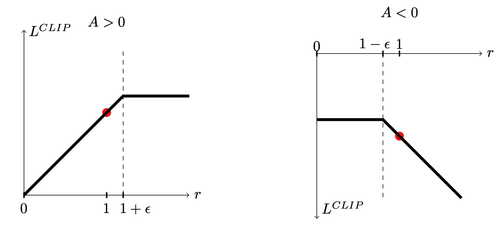
The intuition is clear from the figure. When $A>0$, the sampled action is better than expected, so PPO encourages the new policy to increase its probability. However, excessively increasing this probability may lead to an overly large policy update. Therefore, when $r>1+\epsilon$, the objective is clipped at $(1+\epsilon)A$, preventing further updates in this direction.

Conversely, when $A<0$, the action is worse than expected, and PPO encourages the new policy to decrease its probability. Similarly, if the probability decreases too much ($r<1-\epsilon$), the objective is clipped at $(1-\epsilon)A$, preventing an excessively large policy change.

In both cases, PPO only clips updates that move the policy too far in the direction encouraged by the advantage. Updates in the opposite direction are not restricted because they do not cause destructive policy changes.

PPO in Practice: A Minimal Continuous-Control Update

The equations above become easier to understand when mapped to a concrete implementation. The following code shows the smallest useful PPO update.

It assumes a continuous action space and a diagonal Gaussian policy. We first define the actor-critic model, then follow one batch of data through action sampling, GAE, and the PPO update.

Each action dimension has its own state-dependent mean and learned standard deviation. The rollout buffer stores the observations, sampled actions, rewards, episode-boundary information, old action log-probabilities, and old value predictions.

1. Define ActorCritic

The actor maps an observation to the parameters of a Gaussian action distribution, while the critic maps the same observation to a scalar state-value estimate. For a $D$-dimensional action, the actor produces

$$\mu_\theta(s)\in\mathbb R^D, \qquad \sigma_\theta\in\mathbb R_{>0}^D.$$

The following minimal model uses separate MLPs for the actor and critic. The mean depends on the current observation. The log standard deviation is a learned parameter with one value per action dimension, but it does not depend on the observation.

import torch
import torch.nn as nn
import torch.nn.functional as F
from torch.distributions import Normal


class ActorCritic(nn.Module):
    def __init__(self, obs_dim, action_dim, hidden_dim=64):
        super().__init__()

        self.actor_mean = nn.Sequential(
            nn.Linear(obs_dim, hidden_dim),
            nn.Tanh(),
            nn.Linear(hidden_dim, hidden_dim),
            nn.Tanh(),
            nn.Linear(hidden_dim, action_dim),
        )

        self.critic = nn.Sequential(
            nn.Linear(obs_dim, hidden_dim),
            nn.Tanh(),
            nn.Linear(hidden_dim, hidden_dim),
            nn.Tanh(),
            nn.Linear(hidden_dim, 1),
        )

        # Learning log(std) is numerically easier than optimizing std directly.
        self.log_std = nn.Parameter(torch.zeros(action_dim))

    def forward(self, obs):
        mean = self.actor_mean(obs)
        std = self.log_std.exp().expand_as(mean)

        dist = Normal(mean, std)
        value = self.critic(obs).squeeze(-1)
        return dist, value

The model can be initialized with

actor_critic = ActorCritic(obs_dim, action_dim)
optimizer = torch.optim.Adam(actor_critic.parameters(), lr=3e-4)

In PyTorch, calling

dist, value = actor_critic(obs)

invokes ActorCritic.forward(obs). If obs has shape [batch_size, obs_dim], then:

• dist.mean has shape [batch_size, action_dim] and represents $\mu_\theta(s)$.
• dist.stddev has shape [batch_size, action_dim] and contains the broadcasted learned vector $\sigma_\theta$.
• value has shape [batch_size] and represents $V_\phi(s)$.

The exponential in self.log_std.exp() guarantees a positive standard deviation. A more expressive actor can predict a state-dependent log_std with another network head, but the state-independent version keeps the example focused on PPO itself.

2. Sample an Action with the Old Policy

During rollout collection, an action and its joint log-probability can be obtained as follows:

with torch.no_grad():
    dist, value = actor_critic(obs)
    action = dist.sample()
    old_log_prob = dist.log_prob(action).sum(dim=-1)

For a multi-dimensional action $a_t=(a_{t,1},\ldots,a_{t,D})$, a diagonal Gaussian assumes conditional independence between action dimensions:

$$\pi_\theta(a_t| s_t) = \prod_{j=1}^{D} \mathcal N \left( a_{t,j}; \mu_{\theta,j}(s_t), \sigma_{\theta,j}^2 \right).$$

Therefore, its joint log-probability is the sum of the per-dimension log-probabilities:

$$\log\pi_\theta(a_t| s_t) = \sum_{j=1}^{D} \log\mathcal N \left( a_{t,j}; \mu_{\theta,j}(s_t), \sigma_{\theta,j}^2 \right).$$

The action, joint log-probability, and value prediction must all be stored before the optimizer changes the network. During the update, these stored quantities represent $\pi_{\theta_{\mathrm{old}}}$ and $V_{\phi_{\mathrm{old}}}$.

For one transition, the rollout buffer conceptually stores

transition = {
    "obs": obs,
    "action": action,
    "reward": reward,
    "terminal": terminated,
    "episode_end": terminated or truncated,
    "old_log_prob": old_log_prob,
    "old_value": value,
    "next_value": next_value,
}

Here, terminal means that the underlying MDP truly ended, while episode_end also includes time-limit truncation. For a truncation, next_value should be evaluated on the final observation before the environment is reset.

3. Compute GAE and Critic Targets

The first step is to compute GAE and the corresponding value targets. This computation is performed without gradient tracking because the rollout is treated as fixed training data during the PPO update.

@torch.no_grad()
def compute_gae(
    rewards,
    terminals,
    episode_ends,
    values,
    next_values,
    gamma=0.99,
    lam=0.95,
):
    advantages = torch.zeros_like(rewards)
    gae = torch.zeros_like(rewards[-1])

    for t in reversed(range(len(rewards))):
        bootstrap_mask = 1.0 - terminals[t].float()
        trace_mask = 1.0 - episode_ends[t].float()

        delta = (
            rewards[t]
            + gamma * bootstrap_mask * next_values[t]
            - values[t]
        )
        gae = delta + gamma * lam * trace_mask * gae
        advantages[t] = gae

    returns = advantages + values
    return advantages, returns

The variable delta is the one-step TD error

$$\delta_t = r_t+\gamma(1-d_t^{\mathrm{terminal}})V_{\phi_{\mathrm{old}}}(s_{t+1}) -V_{\phi_{\mathrm{old}}}(s_t),$$

and the backward recursion

$$\hat A_t = \delta_t +\gamma\lambda(1-d_t^{\mathrm{episode}})\hat A_{t+1}$$

is an efficient implementation of the GAE sum. bootstrap_mask decides whether the TD target may use the next-state value. trace_mask prevents the recursive advantage from leaking into the next reset episode. (Here a trace of reward is a rollout buffer that may contains multiple episodes.) They are the same for a true terminal state, but differ for a time-limit truncation: the truncated transition may bootstrap from its final observation, while the GAE trace must still stop at the episode boundary.

The function returns two different training signals:

• advantages[t] tells the actor whether the sampled action was better or worse than the critic expected.
• returns[t] = advantages[t] + values[t] is the regression target used to train the critic.

Before optimization, a rollout with shape [rollout_steps, num_envs, ...] is usually flattened into a batch with shape [rollout_steps * num_envs, ...]. The observations and actions keep their final feature dimension, while log-probabilities, advantages, and returns become one-dimensional arrays.

4. Re-evaluate Stored Actions and Update the Networks

Once the advantages and returns have been computed, the same rollout is shuffled and reused for a small number of minibatch epochs:

def ppo_update(
    actor_critic,
    optimizer,
    obs,
    actions,
    old_log_probs,
    advantages,
    returns,
    *,
    clip_eps=0.2,
    value_coef=0.5,
    entropy_coef=0.01,
    update_epochs=4,
    minibatch_size=64,
    max_grad_norm=0.5,
    target_kl=0.01,
):
    # The rollout targets must remain fixed throughout all update epochs.
    old_log_probs = old_log_probs.detach()
    advantages = advantages.detach()
    returns = returns.detach()

    advantages = (advantages - advantages.mean()) / (
        advantages.std(unbiased=False) + 1e-8
    )

    num_samples = obs.shape[0]
    last_metrics = {}

    for _ in range(update_epochs):
        permutation = torch.randperm(num_samples, device=obs.device)
        epoch_kls = []

        for start in range(0, num_samples, minibatch_size):
            idx = permutation[start : start + minibatch_size]

            dist, values = actor_critic(obs[idx])
            # Sum over action dimensions to obtain one joint log-probability
            # and one joint entropy value for each transition.
            new_log_probs = dist.log_prob(actions[idx]).sum(dim=-1)
            entropy = dist.entropy().sum(dim=-1).mean()

			# get r_{\theta'}
            log_ratio = new_log_probs - old_log_probs[idx]
            ratio = log_ratio.exp()

            unclipped = ratio * advantages[idx]
            clipped = torch.clamp(ratio, 1.0 - clip_eps, 1.0 + clip_eps)
            clipped = clipped * advantages[idx]
            
            # the minus here is because we want gradient ascent
            policy_loss = -torch.min(unclipped, clipped).mean()

            value_loss = 0.5 * F.mse_loss(values, returns[idx])
            loss = policy_loss + value_coef * value_loss - entropy_coef * entropy

            optimizer.zero_grad()
            loss.backward()
            torch.nn.utils.clip_grad_norm_(actor_critic.parameters(), max_grad_norm)
            optimizer.step()

            with torch.no_grad():
                approx_kl = ((ratio - 1.0) - log_ratio).mean()
                clip_fraction = ((ratio - 1.0).abs() > clip_eps).float().mean()
                epoch_kls.append(approx_kl)

                last_metrics = {
                    "policy_loss": policy_loss.item(),
                    "value_loss": value_loss.item(),
                    "entropy": entropy.item(),
                    "approx_kl": approx_kl.item(),
                    "clip_fraction": clip_fraction.item(),
                }

        # Clipping is not a hard trust-region constraint, so KL is still monitored.
        if target_kl is not None and torch.stack(epoch_kls).mean() > target_kl:
            break

    return last_metrics

The inputs to ppo_update have the following roles:

• obs contains the states collected by the old policy.
• actions contains the exact Gaussian samples executed in those states. The actions are not resampled during optimization.
• old_log_probs contains the joint action log-probabilities saved during rollout collection.
• advantages contains the fixed GAE estimates used by the actor.
• returns contains the fixed value targets used by the critic.

At the beginning of each minibatch, actor_critic(obs[idx]) uses the latest parameters to create a new Gaussian distribution. Calling dist.log_prob(actions[idx]) then asks: under the current policy, how likely are the exact actions selected by the old policy? This old-versus-new comparison is what makes the probability ratio possible.

5. Read the Update Line by Line

The implementation contains the full PPO logic in a few operations:

1. old_log_probs are the log-probabilities recorded when the rollout was collected. They are detached and frozen, so they always represent $\pi_{\theta_{\mathrm{old}}}$ during the update.
2. new_log_probs are recomputed after every parameter update and represent the changing policy $\pi_\theta$. For a diagonal Gaussian, dist.log_prob(actions) returns one log-probability per action dimension, so these values must be summed before the probability ratio is computed.
3. Subtracting the two joint log-probabilities and exponentiating gives the importance ratio:

$$r_t(\theta) = \exp\left( \log\pi_\theta(a_t\mid s_t) - \log\pi_{\theta_{\mathrm{old}}}(a_t\mid s_t) \right).$$

4. torch.min(unclipped, clipped) implements the pessimistic surrogate objective. The minus sign converts policy-objective maximization into a loss that can be minimized by a standard optimizer.
5. The value loss trains the critic toward $\hat V_t^{\mathrm{target}}=\hat A_t+V_{\phi_{\mathrm{old}}}(s_t)$.
6. The entropy bonus rewards a less concentrated action distribution and helps prevent exploration from collapsing too early.
7. Advantage normalization changes the scale of the sampled gradient but not which samples have positive or negative advantage. It is a common stabilization technique rather than part of the theoretical PPO objective.

The three loss terms update different parts of the model:

$$L^{\mathrm{total}} = L^{\mathrm{policy}} +c_vL^{\mathrm{value}} -c_e\mathcal H(\pi_\theta).$$

• policy_loss updates the Gaussian actor through mean and log_std.
• value_loss updates the critic toward the GAE-based returns.
• The entropy term discourages the Gaussian standard deviation from collapsing too early.

The negative sign in policy_loss and the negative entropy term come from using a minimization-based optimizer. Mathematically PPO maximizes the clipped objective and entropy, but PyTorch’s optimizer minimizes loss.

The rollout is reused for several epochs because environment interaction is expensive. However, after each optimizer step, the policy moves farther from the policy that generated the data. Too many epochs therefore make the batch increasingly off-policy. approx_kl and clip_fraction are useful diagnostics: a large approximate KL indicates a large overall policy update, while a large clip fraction means that many sampled ratios lie outside $[1-\epsilon,1+\epsilon]$. Early stopping on KL provides an additional safeguard because clipping alone does not guarantee that the new policy remains inside a fixed trust region.

Expand to see details on KL approximation

The approx_kl is obtained with a trick from the original author of PPO (see this blog).

$$D_{KL}(p \| q) = \mathbb{E}_{p} \left[\log \frac{p}{q} \right]$$

We can only use Monte-Calo to estimate this value. The most straight forward way is to use $\log p - \log q$ as estimator. This estimator is unbiased (obviously). But it has great variance since half of the sample is negative, whereas KL-divergence is always positive.

So here we introduce a substitute estimator $r - 1 - \log r$, where $r = q/p$. Taking expectation over this form,

$$\begin{aligned} \mathbb{E}_{p}\left[r - 1 + \log r\right] &= \mathbb{E}_{p}\left[r\right] 1 -\mathbb{E}_{p}\left[\log r\right] \\ &= \int p(x) \frac{q(x)}{p(x)}dx - 1 + D_{KL}(p \| q) \\ &= D_{KL}(p \| q) \end{aligned}$$

So $r - 1 - \log r$ is unbiased estimator for KL-divergence, and you can easily prove that it’s always positive, hence smaller variance

After ppo_update finishes, the rollout should be discarded. A new rollout is then collected using the updated policy, its log-probabilities and value predictions are stored as the new “old” quantities, and the process repeats.

6. Bounded Actions: One Important Omission

One practical detail is omitted from the minimal code above: many continuous-control environments require bounded actions. Directly clipping a Gaussian sample to the environment bounds changes the executed action distribution but not the stored Gaussian log-probability, making the PPO ratio inconsistent. A common solution is to sample an unconstrained Gaussian variable $u_t$, transform it with $a_t=\tanh(u_t)$, scale it to the environment bounds, and include the transformation’s Jacobian correction when computing $\log\pi_\theta(a_t | s_t)$. PyTorch’s TransformedDistribution can handle this consistently. The old and new log-probabilities must always be computed for the same transformed action distribution.