Table of Contents

Open Table of Contents

• Problem Formulation
• Variational Autoencoder
  • Evidence Lower Bound
  • Architecture & Optimization
• Diffusion Models
  • DDPM
  • ELBO for HVAE
  • DDIM

Problem Formulation

For a given set of images $x$, we want the generative model to find the underlying distribution $p(x)$ of all images. Then we sample from $p(x)$ to get a new image $x^{\prime}$ that is unseen in the training datasets, but conform to the “overall nature” of the trained images. So the whole generation process can be thought of as mapping a distribution and then sampling from the distribution.

Conditional generation aims to map a distribution for latent feature $p(z)$ to the image distribution $p(x)$. The model itself can be think of as a function $p(x|z)$. Another question is: how to model the resemblance between distribution. One way is to use KL divergence:

$$\mathcal{D}_{\mathrm{KL}}(p\Vert q) = \int_xp(x) \log\frac{p(x)}{q(x)}\text{d}x$$

And we can simplify the KL divergence into a “likelihood” term with simple math:

$$\begin{aligned} \mathcal{D}_{\mathrm{KL}} (p_{\mathrm{data}}\Vert p_{\theta}) &= \sum_x p_{\mathrm{data}}(x) \log\frac{p_{\mathrm{data}}(x)}{p_{\theta}(x)} \\ &= \sum_x -p_{\mathrm{data}}(x)\log{p_{\theta}(x)} + C \\&= -\mathbb{E}_{x\sim p_{\mathrm{data}}}\log{p_\theta(x)} + C\end{aligned}$$

We want to minimize $\mathcal{D}_{\mathrm{KL}} (p_{\mathrm{data}}\Vert p_{\theta})$ in parameter space $\theta$, which is equivalent to maximize $\mathbb{E}_{x\sim p_{\mathrm{data}}}\log{p_\theta(x)}$. We can interoperate the term as “maximum likelihood”, which has an intuitive explanation of maximizing the possibility of observing the ground-truth data from latent distribution.

Variational Autoencoder

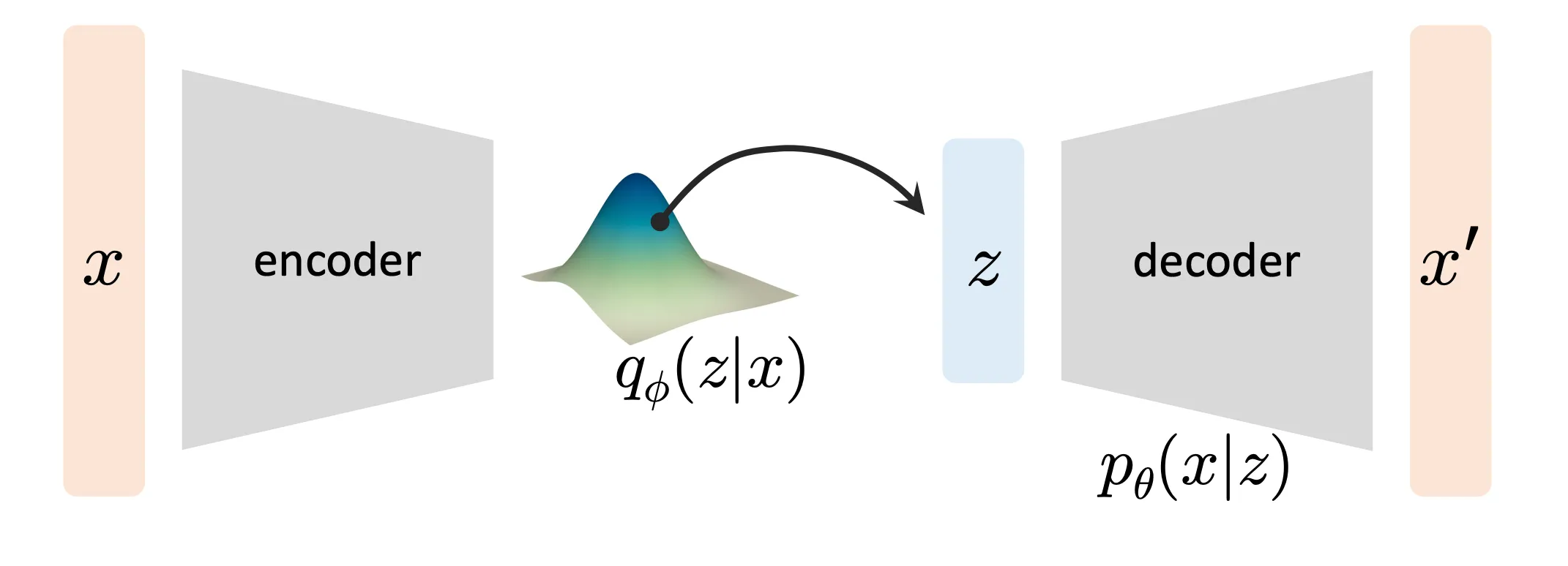
It is very hard to directly model the distribution for image, and even if we can model such a distribution directly with a neural network, we have no idea how to sample from it. Variational autoencoder model the problem by introducing a latent space. If we impose the latent space $q(z)$ to be a fixed distribution (e.g. normal distribution) and somehow find the mapping from this latent distribution to image distribution, we only need to sample from this simple distribution and map the sample to image space to get the final generated image. We can think of the mapping as a function to be optimized $p_\theta(x| z)$.

Evidence Lower Bound

So now we can rephrase our objective function and see how can we optimize the mapping.

$$\begin{aligned} \log{p_\theta(x)} &= \int q(z)\log p_{\theta}(x)\text{d}z \quad \quad \quad \quad\quad\quad\quad \text{\small{(Law of Total Probability)}}\\ &= \int q(z)\log \frac{p_{\theta}(x|z) p(z)}{p_{\theta}(z|x)}\text{d}z \quad\quad\quad\quad\space\text{\small{(Baye's Rule)}} \\ &= \int q(z)\log \frac{p_{\theta}(x|z) p(z)}{p_{\theta}(z|x)} \frac{q(z)}{q(z)}\text{d}z \\ &= \mathbb{E}_{z\sim q(z)} \left[\log p_\theta(x|z)\right]-\mathcal{D}_{\text{KL}}(q(z)\Vert p(z)) +\mathcal{D}_{\text{KL}}(q(z)\Vert p_\theta(z|x)) \end{aligned}$$

Notice that the $q(z)$ here is an arbitrary distribution over $z$, $p(z)$ is the pre-determined latent distribution. To make this expression more interpretable, we let the $p(z)$ to be a parameterized posterior $q_\phi(z|x)$ of the latent value.

But why do we do this? It’s because we must have some training objective. VAE is deterministic probability transition model (different from diffusion method ddpm we will introduce later), which means that a sample from a latent space must correspond to a sample in the image space. If we directly assign $q(z)$ to be a Gaussian, we will have to manually assign the correspondence between Gaussian noise to generated image. Instead, we choose to model $q(z)$ to be the posterior, and let a neural network learn the correspondence itself.

So $\log{p_\theta(x)}$ can be expressed as:

$$\mathbb{E}_{z\sim q(z)} \left[\log p_\theta(x|z)\right]-\mathcal{D}_{\text{KL}}(q_\phi(z|x)\Vert p(z)) +\mathcal{D}_{\text{KL}}(q_\phi(z|x)\Vert p_\theta(z|x))$$

Notice that the third term measure the difference between ground-truth posterior and predicted posterior, which is intractable because we don’t know anything about ground-truth posterior $p_\theta(z|x)$. But we notice that KL divergence will always be positive. So we turn to optimize the following value, which is called ELBO (Evidence Lower BOund):

$$\mathbb{E}_{z\sim q_\phi(z|x)}\left[\frac{p_\theta(x,z)}{q_\phi(z|x)}\right]= \mathbb{E}_{z\sim q(z)} \left[\log p_\theta(x|z)\right]-\mathcal{D}_{\text{KL}}(q_\phi(z|x)\Vert p(z))$$

The moved-to-left term $\mathcal{D}_{\text{KL}}(q(z)\Vert p_\theta(z|x))$ tells us that we are actually compromising the resemblance between predicted posterior and the ground-truth posterior when we are optimizing over ELBO.

The remaining two terms is also very meaningful. The $\mathbb{E}_{z\sim q(z)} \left[\log p_\theta(x|z)\right]$ term is a reconstruction loss. Maximize the term means maximizing the likelihood of observed training data. The $\mathcal{D}_{\text{KL}}(q(z)\Vert p(z))$ is regularization loss. Minimizing this term means bringing the predicted latent distribution closer to our pre-assigned normal latent distribution. We will see in later section why this is useful.

Architecture & Optimization

VAE designs a wonderful network structure that allows us to jointly optimize $\theta, \phi$. The neural encoder outputs the mean and diagonal covariance of the latent normal and the latent prior is often selected to be a standard multivariate Gaussian

$$q_\phi(z|x) = \mathcal{N}(z;\mu_\phi(x), \sigma^2_\phi(x)\mathbf{I})\\ p(z) = \mathcal{N}(z;0, \mathbf{I})$$

Network Design of VAE. (Image Source from here)

The objective can be easily transformed to target loss.

For the reconstruction loss $\mathbb{E}_{z\sim q(z)} \left[\log p_\theta(x|z)\right]$, we take its opposite number so that we can minimize it . Firstly, we use one-step Monte Carlo sampling to get rid of the expectation. Then we model the predicted $p_\theta(x|z)$ to be Gaussian with fixed variance $\mathcal{N}(x|x^{\prime},\sigma_0)$. Then the loss term is simply $1/2\sigma \Vert x - x^{\prime} \Vert ^ 2 + C$. We can substitute it we L2 loss.

Regularization loss $\mathcal{D}_{\text{KL}}(q(z)\Vert p_\theta(z))$ can be calculated with simple math:

$$\begin{aligned}&\quad\mathcal{D}_{\text{KL}}(q(z)\Vert p(z)) \\ &= -\int_z \frac{(z - \mu)^2}{2\sigma^2} \mathcal{N}(\mu, \sigma^2) \, dz + \int_z \frac{z^2}{2} \mathcal{N}(\mu, \sigma^2) \, dz - \int_z \log \sigma \mathcal{N}(\mu, \sigma^2) \, dz \\ &= -\frac{\mathbb{E}[(z - \mu)^2]}{2\sigma^2} + \frac{\mathbb{E}[z^2]}{2} - \log \sigma \\ &= \frac{1}{2} \left( -1 + \sigma^2 + \mu^2 - \log \sigma^2 \right)\end{aligned}$$

Diffusion Models

In VAE, we choose to model the transition function from $p(z)$ to $p(x)$ with a single neural network. But the transition is too hard for a single network to directly learn. Diffusion model adopts a more progressive transition. One famous interpretation for diffusion model is Hierarchical-VAE.

We spilt the whole transition into a lot of intermediate stages. At the same time, we assign each intermediate state to be a fixed distribution (To be precise, conditional intermediate state). The HVAE we get from the assumption is: DDPM.

DDPM

In essence, we want to model the process of “slowly” turning a Gaussian distribution $p(z)$ into an image distribution $p(x)$. But at first, let us take a step back and consider how to turn an image distribution $p(x)$ into a Gaussian distribution $p(z)$.

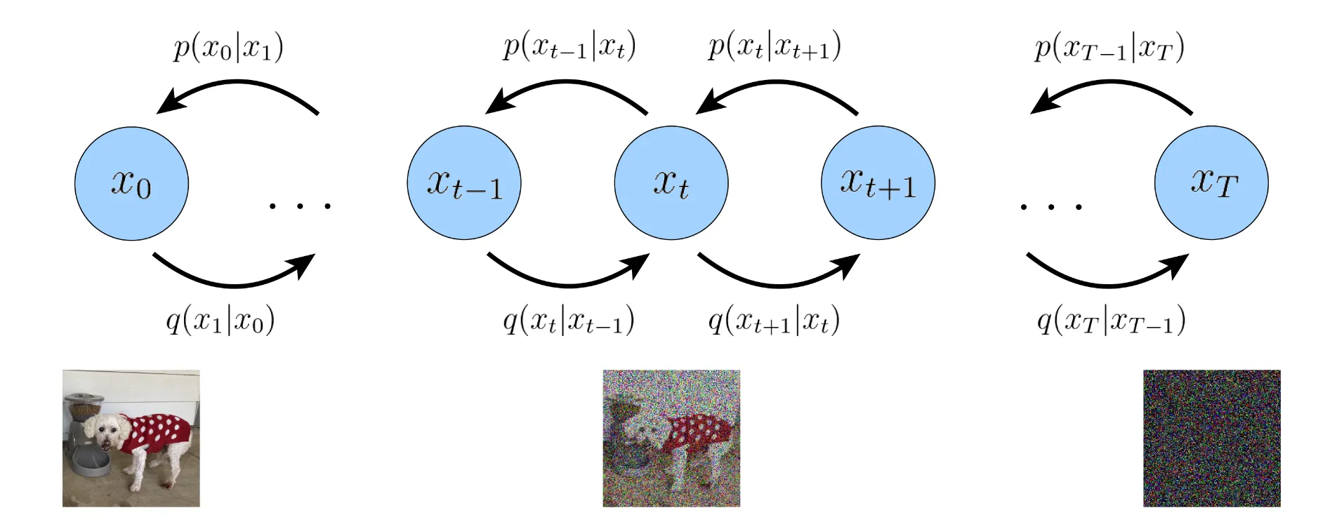
We want to achieve this through gradually adding noise to the image until it becomes pure Gaussian noise. We model the process as a Markovian process.

Noisifying and denoiding process of DDPM (Image Source from Luo et al. 2022)

For simplicity and uniformity, we let $p(x)$ to be $p(x_0)$ and the latent distribution $p(z)$ to be $p(x_T)$. We let the transition function $q(x_t | x_{t-1})$ to be:

$$x_t = \sqrt{\alpha_t}x_{t-1} + \sqrt{1-\alpha_t}\epsilon_{t-1} \quad \epsilon_t \sim \mathcal{N}(0,\mathbf{I})$$

The reason we want to choose such a strange coefficient is that we want to preserve the variance of the random variable.

With simple math, we can easily get the distribution for each intermediate state under the condition of initial image $p(x_t| x_0)$:

$$x_t \sim \mathcal{N}(\sqrt{\bar{\alpha}_t}x_0, (1-\bar{\alpha}_t)\mathbf{I} )$$

Notice that we $\alpha_t$ is a pre-assigned coefficient, hence the $\bar{\alpha}_t$ is pre-assigned. Letting $\bar{\alpha}_T$ take the value of 0, and we can get the final Gaussian latent distribution.

$$p(x_{t-1}|x_t) = \frac{q(x_t|x_{t-1})p(x_{t-1})}{p(x_t)}$$

Now that we know how to turn $p(x_0)$ to $p(x_T)$, we simply need to reverse the process to turn $p(x_T)$ to $p(x_0)$, this is where the Bayes’ Rule comes to rescue. For each intermediate step:

The equation is intractable, because we don’t know $p(x_{t-1})$ and $p(x_t)$. But we do know $p(x_{t-1}|x_0)$ and $p(x_{t}|x_0)$. So we can turn to calculate:

$$p(x_{t-1}|x_t,x_0) = \frac{q(x_t|x_{t-1},x_0)p(x_{t-1}|x_0)}{p(x_t|x_0)}$$

We know the interpretable representation of all 3 terms on the right side of the equation, so we can directly calculate the conditional posterior $p(x_{t-1}| x_t,x_0)$:

$$\mathcal{N}\left(\underbrace{\frac{\sqrt{\alpha_t} (1 - \bar{\alpha}_{t-1}) \, x_t + \sqrt{\bar{\alpha}_{t-1}} (1 -\alpha_t) \, x_0}{1 - \bar{\alpha}_t}}_{\mu_{t-1}(x_t,x_0)}, \underbrace{\frac{(1 - \alpha_t)(1 - \bar{\alpha}_{t-1})}{1 - \bar{\alpha}_t} \, \mathbf{I}}_{\Sigma_{t-1}}\right)$$

We get the distribution from rigid math, sample from this distribution and taking iterative steps back, we have accomplished the task!

But notice that what we get is $p(x_{t-1}| x_t,x_0)$, but during inference, we don’t know the $x_0$(this is actually the image we want to generate). This is where the neural network comes to help. We train a gigantic leap, and train a neural network that predict $x_0$ from $x_t$.

Notice that $p(x_t | x_0)$ is a Gaussian, so we can use $x_t$ to interpret $x_0$ with simple reparameterization.

$$x_0 = \frac{1}{\sqrt{\bar{\alpha}_t}}(x_t - \sqrt{1-\bar{\alpha}_t}\epsilon_0)$$

Previous work has empirically shown that predicting the noise $\epsilon_0$ is better than predicting $x_0$. We parameterize $\epsilon_0$ to be $\epsilon_\theta(x_t, t)$. And the distribution $p(x_{t-1}|x_t,x_0)$ becomes:

$$\mathcal{N}\left(\underbrace{\frac{1}{\sqrt{\alpha_t}}x_t-\frac{1-\alpha_t}{\sqrt{1-\bar{\alpha}_t}\sqrt{\alpha_t}}\epsilon_\theta(x_t, t)}_{\mu_{t-1}(x_t, t)}, \underbrace{\frac{(1 - \alpha_t)(1 - \bar{\alpha}_{t-1})}{1 - \bar{\alpha}_t} \, \mathbf{I}}_{\Sigma_{t-1}}\right)$$

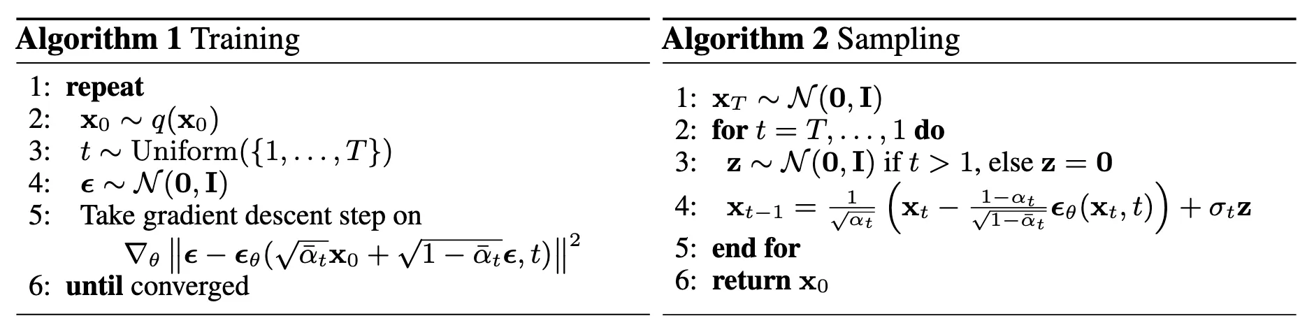
So the overall training and inference procedure is:

Pseudo-code for training and inferencing process. (Image Source from Ho et al. 2020)

ELBO for HVAE

We have known from the last section that we can approximate the posterior transition distribution with a neural network that predict original image $x_0$ from $x_t$ and $t$. But does this really help with our ultimate goal of maximizing log likelihood $\mathbb{E}_{x\sim p(x)}[-\log{p_\theta(x)}]$? We can actually derive a closed form ELBO with the assumption we made. (Please refer to this paper for a detailed derivation.)

$$\log{p(\boldsymbol{x})} \geq \underbrace{\mathbb{E}_{q(\boldsymbol{x}_1|\boldsymbol{x}_0)}[\log p_{\boldsymbol{\theta}}(\boldsymbol{x}_0|\boldsymbol{x}_1)]}_{\text{reconstruction terrm}}-\underbrace{D_{\mathrm{KL}}(q(\boldsymbol{x}_T|\boldsymbol{x}_0)\parallel p(\boldsymbol{x}_T))}_{\text{prior matching term}}\\-\sum_{t=2}^T\underbrace{\mathbb{E}_{q(\boldsymbol{x}_t|\boldsymbol{x}_0)}\left[D_{\mathrm{KL}}(p(\boldsymbol{x}_{t-1}|\boldsymbol{x}_t,\boldsymbol{x}_0)\parallel p_{\boldsymbol{\theta}}(\boldsymbol{x}_{t-1}|\boldsymbol{x}_t))\right]}_{\text{denoising matching terrn}}$$

We can notice that each term of the ELBO has its specific meaning.

• The reconstruction term measure the expected likelihood of the predicted reconstructed image. This term is jointly optimized with Monte Carlo estimate.
• The prior matching term tries to keep the final notified latent space as close as possible. It contains no trainable parameter, and by carefully selecting the noising parameter $\alpha$, we can diminish the term to zero.
• The denoising matching term is the primary part of the ELBO. The term aims to keep the predicted distribution to align with the ground-truth conditional posterior distribution as closely as possible.

We have proved in the last section that $p(x_{t-1}|x_t,x_0)$ is a normal distribution. Now suppose $p_\theta(x_{t-1}|x_t)$ is a normal distribution $\mathcal{N}(\mu_t(x_t,x_0), \sigma_{t-1}^2\mathbf{I})$. Then we have:

$$\begin{aligned}&\underset{\boldsymbol{\theta}}{\operatorname*{\operatorname*{\arg\min}}}D_{\mathrm{KL}}(q(x_{t\boldsymbol{-}1}|x_t,x_0)\parallel p_{\boldsymbol{\theta}}(x_{t\boldsymbol{-}1}|x_t))\\=&\arg\min_{\boldsymbol{\theta}}\frac{1}{2\sigma_t^2}\frac{(1-\alpha_t)^2}{(1-\bar{\alpha}_t)\alpha_t}\left[\left\|\epsilon_0-\epsilon_{\theta}(x_t,t)\right\|_2^2\right]\end{aligned}$$

The optimizing objective align with the loss function we choose in the last section(discarding all the coefficients, which was empirically shown better in the original paper).

DDIM

Now let’s talk about DDIM. Notice that during the training process, we never directly use the transition $p(x_t | x_{t-1})$. This means that we actually never assume the forward(adding noise) process to be Markovian (Although we do derive most of the equation from a Markovian forward process). The only condition used during forwarding process is that the conditional distribution of $x_t$ is a normal distribution:

$$x_t \sim \mathcal{N}(\sqrt{\bar{\alpha}_t}x_0, (1-\bar{\alpha}_t)\mathbf{I} )$$

We can also notice that during the backward (denoising) process, the only distribution we sample from is $p(x_{t-1}| x_t,x_0)$. Under the Markovian assumption $p(x_{t-1}| x_t,x_0)= p(x_{t-1}| x_t)$. But this is not necessarily true for non-Markovian forwarding process. But we can still derive a family of posterior distribution $p_\sigma(x_{t-1}| x_t,x_0)$ indexed by a vector $\sigma$ with dimension $t$ . (This can be proved with method of undetermined coefficients. )

$$p_\sigma(x_{t-1} | x_t, x_0) = \mathcal{N} \left( \sqrt{\bar{\alpha}_{t-1}} x_0 + \sqrt{1 - \bar{\alpha}_{t-1} - \sigma_t^2} \cdot \frac{x_t - \sqrt{\bar{\alpha}_t} x_0}{\sqrt{1 - \bar{\alpha}_t}}, \sigma_t^2 \mathbf{I} \right)$$

Notice that if we let $\sigma_t = \frac{(1 - \alpha_t)(1 - \bar{\alpha}_{t-1})}{1 - \bar{\alpha}_t}$, the forwarding process becomes Markovian and the posterior distribution becomes that of DDPM’s.

And following the same steps, we train a neural network to predict $x_0$($\epsilon_0$) from $x_t$ and $t$. Taking in the reparameterization of $x_0$, we get the following distribution to sample from $p_\sigma(x_{t-1}| x_t,x_0)$.

$$\mathcal{N} \left( \frac{\sqrt{\bar{\alpha}_{t-1}}}{\sqrt{\bar{\alpha_t}}}x_t + \left( \sqrt{1-\bar{\alpha}_{t-1} - \sigma_t^2} - \frac{\sqrt{\bar{\alpha}_{t-1}}\sqrt{1-\bar{\alpha}_{t}}}{\sqrt{\bar{\alpha}_{t}}} \right)\epsilon_0, \sigma_t^2 \mathbf{I}\right)$$

Another good property that DDIM has is that we can drastically accelerate the inference process:

As the denoising objective $L1$ does not depend on the specific forward procedure, as long as $q_\sigma(x_t|x_0)$ is fixed, we may also consider forward processes with lengths smaller than $T$.

Since any forwarding process with the conditional normal distribution property can be applied to the training procedure. It certainly includes denoising process with less time-steps. We can choose these sub-sequence as our inference sequence to accelerate the inference process. (Notice that this property also applies to the DDPM inference algorithm, since DDPM is only an instance of DDIM).

Specifically, given a sequence of intermediate states $(x_{\tau_1}, \dots x_{\tau_S})$, where $\tau$ is a sub-sequence of the original time-steps $[1,\dots, T]$. The posterior transition distribution $p_\sigma(x_{\tau_{t-1}}| x_{\tau_t},x_0)$ can be modeled as:

$$\mathcal{N} \left( \frac{\sqrt{\bar{\alpha}_{\tau_{t-1}}}}{\sqrt{\bar{\alpha}_{\tau_t}}}x_{\tau_t} + \left( \sqrt{1-\bar{\alpha}_{\tau_{t-1}} - \tilde{\sigma}_{\tau_t}^2 } - \frac{\sqrt{\bar{\alpha}_{\tau_{t-1}}}\sqrt{1-\bar{\alpha}_{\tau_t}}}{\sqrt{\bar{\alpha}_{\tau_t}}} \right)\epsilon_0, \tilde{\sigma}_{\tau_t}^2 \mathbf{I}\right)$$

Notice that in DDIM, only $\bar{\alpha}_t$ is preassigned, any other notations need to be derived from $\bar{\alpha}_t$. For DDPM, we have $\sigma_t = \frac{(1 - \alpha_t)(1 - \bar{\alpha}_{t-1})}{1 - \bar{\alpha}_t} = \frac{(1 - \bar{\alpha}_t/\bar{\alpha}_{t-1})(1 - \bar{\alpha}_{t-1})}{1 - \bar{\alpha}_t}$. So the variance $\tilde{\sigma}_{\tau_t}$ should take the form of:

$$\tilde{\sigma}_{\tau_t} = \frac{(1 - \bar{\alpha}_{\tau_t}/\bar{\alpha}_{\tau_{t-1}})(1 - \bar{\alpha}_{\tau_{t-1}})}{1 - \bar{\alpha}_{\tau_t}}$$